Interactive Computing with Jupyter Notebooks
What is Interactive Computing?
Interactive computing is a fancy term for programming where we issue commands to a running program and get results right away.
Examples of Interactive Computing:
- spreadsheet applications
- REPL (Read Eval Print Loop): interactive language shells
- editor plugins that run the code or tests as we type and display results
- Jupyter Notebooks and alternatives
The advantage of interactive computing is that we get all the intermediate results before arriving at a final solution. This is especially useful in situations where we are not sure what the end result looks like and so we develop things step by step, basing our next step on the result of the previous one.
What is Jupyter Notebook?
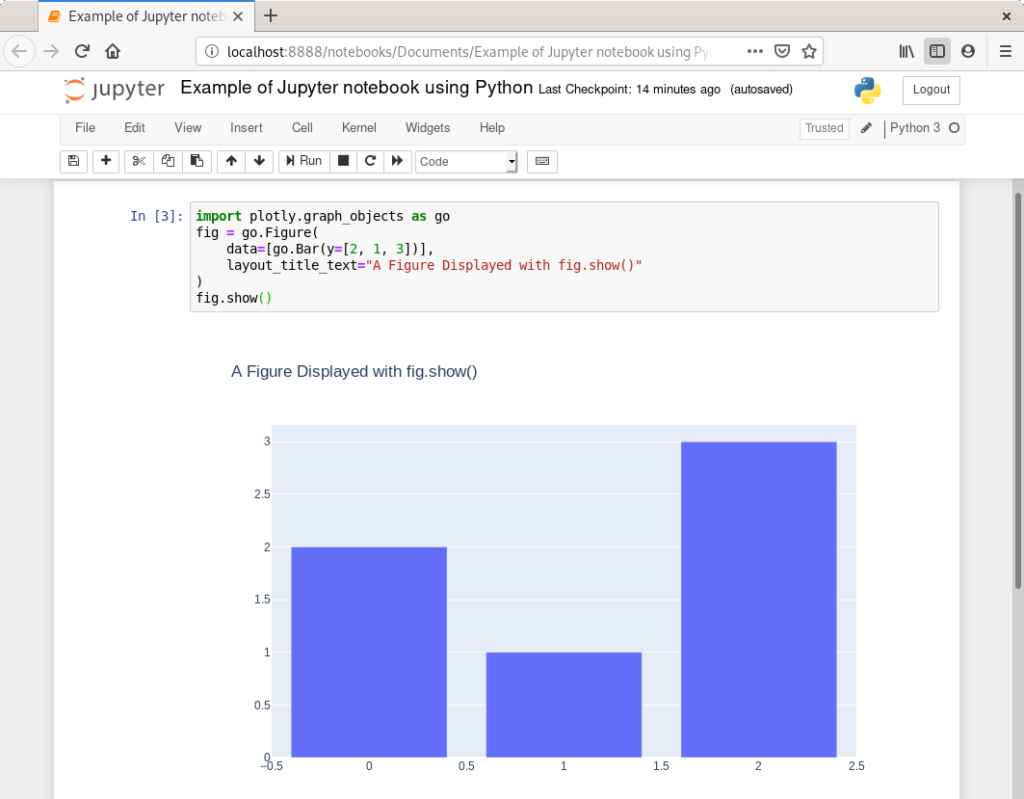
In short, Jupyter Notebook is an interactive computing environment that mixes code, results of running the code in graphical form and documentation in one document. It consists of series of blocks (code, results, documentation) and the result is an interactive or non-interactive document, not a program.
Jupyter Notebooks can be created, opened and viewed in Jupyter Notebook App, the primary application used to work with this documents. We can recognize a Jupyter Notebook document based on the file extension, which is .ipynb.

What can we use Jupyter Notebooks for?
There are two main use cases:
- Developing a piece of code, a solution, an algorithm interactively
- Documenting the development and thinking process that led to such a piece of code or solution
The fact that we can play around a lot, seeing even graphical results along the way led Jupyter Notebooks to be super popular among data analysts, data scientists and machine learning developers.
The second use case is also very important. We can easily share the finished (or unfinished) notebooks for educational purposes. As notebooks can be easily modified later and code re-executed, it creates a perfect learning environment. It can be also used for assignments, where some blocks can be left empty or incomplete for others to fill.
Installation & setup
Technically, Jupyter Notebooks are just files and so we need a program to work with them. That program is called Jupyter Notebook App. Jupyter Notebook App is basically a web-based application and so we typically use it in the browser. It is separated into client and server part behind the scenes, but this is not so important now. When we run it, it will run the server in the background and open a browser window with the notebook itself.
We can install it by installing Anaconda distribution, which is a collection of scientific tools for data science that includes it.
If we want to install just Jupyter Notebooks we can do so via pip, Python package manager. Pip should come with our Python distribution, so all we need to do is to install Python. On Linux system, Python, and therefore pip, will be installed already.
Then to install Jupyter, just run this on the command line:
pip install jupyter
Official installation instructions can be found on the Install page.
The application itself, Jupyter Notebook App, can be started from the command line:
jupyter notebook
To open a specific notebook file, add a parameter with the file’s path:
jupyter notebook notebook.ipynb
How to work with Jupyter Notebooks?
The whole application is graphical and so pretty easy to use. There are also plenty of tutorials and Youtube videos around to help us.
The important thing that is worth mentioning are kernels. Kernels are the background computing resources that we can use in our notebooks, depending on what kind of computation or programming we want to do. So Python 3 would be a kernel to develop solutions in Python, but today we can install more kernels and so work with variety of computing environments.
Example notebooks
A gallery of interesting Jupyter Notebooks on Github provides a great way to get inspired and see what is possible!
I really recommend giving Jupyter Notebooks a shot. It can fill a lot of gaps and make development or learning much easier.
Last updated on 24.8.2019.